

ROI Analysis Report
Objective of the Analysis
Use data from the firm’s accounting and compensation systems to quantitatively estimate the impact of CCD’s Business Development Program for Partners on the participant’s success in generating client revenue for the firm.
Executive Summary
The data and statistical analysis demonstrate that, on average, the CCD Business Development Program led to at least $244,000 additional revenue per year per participant for four years from the program start, for a total of $976,000 additional revenue per participant. This estimate comes from comparing the increase in participants’ revenue credits before the program to four years after the start of the program versus the increase in revenue credits over the same period for a set of partners with the same practice group, tenure, and revenue credit profiles as the participants. In addition, comparing the samples’ median revenue suggests that the increase was broad-based across most participants rather than being driven by a few high-performing stars. Finally, participants drop out of the data at a lower rate than the non-participants, demonstrating that the BD program may contribute to higher partner retention rates. (Full Executive Summary)
Background
The CCD Business Development Programs for Partners that was delivered to this AmLaw 50 ranked client consisted of two separate in-person training sessions totaling 2.5 days. Each attorney was assigned a CCD individual consultant that worked with them by telephone once a month for 1.5 hours over 15 months (on average).
Each cohort of participants included 10 to 12 attorneys who participated in program activities for up to 18 months. The first cohorts began the program in 2007; the last cohorts started in 2014. The firm reviewed and evaluated the BD program in 2011 and then renewed and extended it for an additional three years. All told, there were 15 cohorts and 171 participants. See Figure 1 for the number of participants each year.
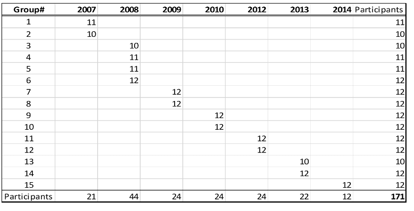
Figure 1 – Number of Program Participants by Cohort (“Group”) and Year
Analytic Approach to Estimating Program Impact
To estimate the program’s impact on participant business development success, we conducted a “difference-in-differences” comparison. This consists of comparing the difference in participants’ success after the program relative to before the program against the difference in success over the same timeframe for a set of non-participants that were as similar as possible to the participants just before the participants started the program.
To implement this approach, we made two important analytical decisions: (1) how to measure business development performance; and (2) to whom to compare the participants.
Performance measure: The program’s goal was to enhance the participants’ skills in developing new business from prospective and existing clients. Business development success means bringing in client revenue. We focused on annual revenue credits. A section in the technical appendix describes the calculation of this measure.
Performance benchmarks: We selected two sets of non-participants: (i) “Contemporaries” who matched the participants on several key characteristics in the year before the participants began the program; and (ii) “Predecessors” whose characteristics in the 2002-2005 period—before the introduction of the program—matched the participants in the year before they began their program.
The following section describes these comparison samples in more detail.
Performance Benchmarks: to whom should we compare the participants?
The key challenge in estimating the effect on the participants is figuring out to whom to compare them. The simplest comparison is “before vs. after” – comparing the participants’ annual revenue after the program to their annual revenue before the program. This is shown in Figure 2, which shows the average annual revenue of all participants three years before vs. three years after the program.
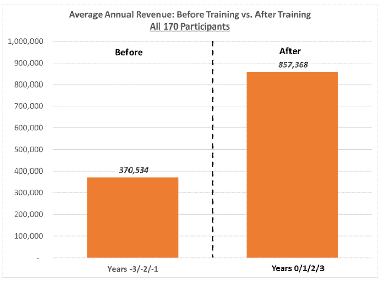
Figure 2 – Participant Revenue Before vs. After Program
However, many participants were relatively new partners with 12-16 years of practice experience. For most new partners, annual revenue increases year over year. The real question is whether the participants’ post-program revenue increased more than we expected in the program’s absence. To form the benchmark of “what we would have expected,” we need a set of attorneys that did not participate in the program but were as similar to the participants as possible. In experimental parlance, we needed to create a “control group” of non-participants to compare to the participants.
“Contemporaries”
Our first comparison set is attorneys that did NOT participate in the program but were similar to the participants on attributes we can observe in the year before the participants started the program. We call this comparison set the “contemporary controls.”
Specifically, for each participant, we identified all non-participants that matched that participant on three attributes in the year before the participant started the program:
- in the same practice group
- tenure as a partner (# of years as a partner)
- annual revenue*
*Note: to match annual revenue, we created seven revenue categories, each with a roughly equal number of partners. A match occurred when the participant and non-participant were in the same revenue category.
The weakness of the “contemporaries” benchmark, however, is that partners were not randomly selected to participate. Participants were chosen because of a perceived potential for being good at business development and because they had not yet demonstrated outstanding business development ability. The participants were different from non-participants on dimensions that are not observable in the firm’s accounting/compensation/timekeeping systems. For instance, if the participants had, on average, better business development aptitude than the non-participants of the same practice/tenure/revenue, then we might expect them to demonstrate greater revenue growth over time even in the absence of participating in the program.
“Predecessors”
To combat the potential “selection effect” in the Contemporaries comparison, we created a second comparison using the data from before the BD program was first instituted in 2007. Specifically, we matched participants to attorneys with similar characteristics from 2002 to 2005, before the program was available, and then used the revenue performance of those “predecessor” attorneys as the benchmark. For instance, imagine a participant in the employment practice who went through the program starting in 2012. In the year before entering the program (2011), this attorney had been a partner for two years, and her annual revenue was in the 2nd revenue category. The “predecessor” comparison set for this attorney is all employment attorneys who, between 2002-2005, were two years as a partner and in the 2nd revenue category. (Note that for these matches, annual revenue was adjusted for the calendar year to account for the average revenue per attorney increased steadily over the 2002-2017 period.)
The idea behind this Predecessor sample is that it includes attorneys who would have been selected to participate in the program but were not because it was not yet available. It is arguably a more apples-to-apples comparison than using the Contemporaries.
Figure 3 summarizes the criteria used to match participants to Contemporary and Predecessor non-participants, as well as how many participants and controls (non-participants) are in each set. Note that each sample excludes many of the 171 total participants. This means that for many of the participants, we could not find a matching non-participant. Participants with “unique” profiles are not used to estimate the program’s impact. Note also that we did NOT match two observable characteristics: gender and geographic office. Requiring matches on these two characteristics, in addition to the first three, vastly reduced the number of matches available for the analysis. Instead, we include these characteristics as control variables in the statistical analyses (see the Technical Appendix for details on the regression models).
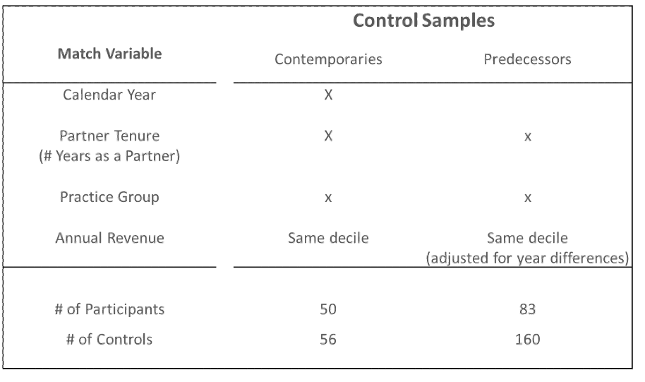
Figure 3 – Criteria for Matching Participants to Non-Participant “Controls”
Estimating the Average Impact
The essence of our estimation of the impact of the program on annual revenue is comparing the difference in the participants’ revenue before vs. after the program to the difference in the non-participants’ revenue over that same time frame; i.e.:
- Impact = { [ (Participant_Revenue_After) – (Participant_Revenue_Before) ] –
- [ (NonParticipant_Revenue_After) – (NonParticipant_Revenue_Before) ] }
To calculate the average revenue before, we use three years before the program’s first year. To calculate the average revenue after, we use the program’s first year and the three years later. We chose a three-year window because that created a consistent timeframe for all the cohorts. The last set of cohorts began in 2014, and we had access to revenue data through 2017, so we could have at most three years of post-program data for all participants. Beyond three years post-program, we start losing both participant and non-participant attorneys from the data, so the comparisons become less consistent the more years after the start of the program we looked at. We discuss this attorney attrition in a later section.
Figure 4 reports the estimated impact using the Contemporary Controls by illustrating the logic of the difference-in-difference method of estimating program impact. Consider first the orange bars labeled “Participants.” The “participants” bar on the left plots the average annual revenue of the 50 matched participants in the three years before entering the program. The “participants” bar on the right plots the average annual revenue of those 50 participants in the year of and the three years after they began the program. For this set of 50 participants, average annual revenue increased from just under $400K per year to just over $800K per year, a growth of about $400K.
The “before vs. after” difference for the “Controls” represents the benchmark revenue growth against which to compare the participants’ revenue growth. The controls went from about $450K annual revenue to just over $600K, a change of about $150K. The participants’ increase of $400K per year was about $250K per year, greater than the benchmark.
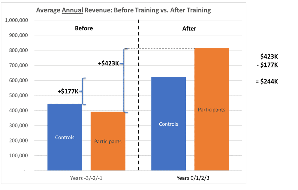
Figure 4 – Quantitative Estimation of Program Impact Using “Difference-in-Difference” with Contemporary Sample
Figure 5 illustrates the same “difference in differences” calculation using the Predecessors sample. Here the participants—in this sample, 83 participants—show an even greater net increase of $288K per year.
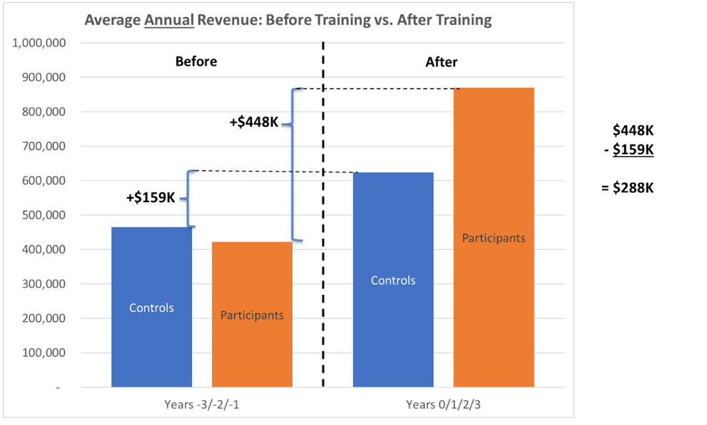
Figure 5 – Quantitative Estimation of Program Impact Using “Difference-in-Difference” with Predecessor Sample
The two methods of comparison—Contemporaries and Predecessors—yield estimates of a similar magnitude: $244K vs. $288K per year. This heightens the degree of confidence in concluding that, on average, the program increased each participant’s annual revenue by about $250,000 per year for four years (the start year + three years after).
Statistical Analyses for Gender & Office adjustments and Confidence Intervals
We use statistical models to generate the estimates in Figures 4 and 5 rather than just calculating the “raw” average revenue for participants and controls. We use these models for two reasons.
- First, as noted earlier, we do not match participants to controls on gender and office. Yet average revenue differs between male and female attorneys and attorneys at different offices. We use regression models to control for differences between the participants and non-participants in the percentage of female attorneys and the distribution across offices.
- Second, the regression models use the variance across individual observations to estimate the confidence interval around the estimated effect (discussed in the next section). In the Technical Appendix, we describe the regression models in more detail.
Intervals: “True” average impact likely to fall between $22K and $481K per year
Each annual revenue bar shown in Figures 4 and 5 represents an average across many attorneys. The actual annual revenue for any one attorney might be much higher or much lower than the average for idiosyncratic reasons that we do not observe (and/or because of chance). In other words, there is variance around each average value. Our estimated impact represents the most likely value but does not guarantee that each attorney participating in the program will generate an extra $250,000—some will generate less, some will generate more.
In addition to estimating the most likely value of the program’s impact, the statistical analysis uses this variance to quantify the probability that the actual impact is higher or lower than that. In particular, the analysis generates 95% confidence intervals: there is a 95% chance that the program’s true impact falls somewhere between the low and high values of the confidence interval. (Said differently: there is a 5% chance that the program’s true impact lies below the lowest value or above the highest value).
Figure 6 plots the 95% confidence intervals for the estimated impact using the contemporaries and predecessors’ samples. It also includes an illustrative probability distribution along the confidence interval range to convey the idea that the average (e.g., $244K) is the most likely value of the impact, and values further away from that are possible but less probable. A key takeaway from this Figure is that the actual program impact could be as low as $22K but as high as $481K per year. At the very least, the confidence intervals indicate an extremely high probability that the program’s impact is positive (i.e., not zero).
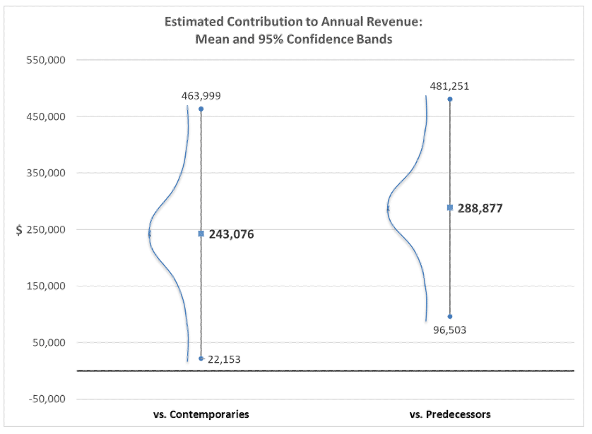
Figure 6 – Confidence Intervals around Estimates of Average Impact
Median Analysis: BD Program lifts all boats; control sample pulled up by outliers
Figures 4 and 5 compare the average revenue of participants vs. controls. We also compared the median revenues to assess whether either group’s average is particularly influenced by outliers with very high (or very low) performance. The median represents the point where there are an equal number of values on either side, so it is not influenced by individual values that are very high or very low in the way that the average can be.
Figure 7 plots the median revenue for participants and controls in the “before” and “after” periods. The figure shows a significant increase for participants, similar to the increase in their average revenue. However, it shows only a very modest increase for the controls, quite a bit less than the increase in the average.
For the participants, the fact that the median closely tracks the mean implies that most participants experienced a substantial increase in revenue—the average revenue increase is not the result of a few high-performing stars. By contrast, for the controls, the fact that the average increases substantially while the median barely increases indicates that many of the attorneys in the control group did not experience a revenue increase, and just a few high-performing attorneys pulled up the average.
This is additional evidence supporting the idea that the BD program enhances participants’ revenue generation skills: the performance increase of the participants is broad-based, as might be expected by the deliberate transmission of skills, rather than attributed to some pre-existing talent of a few outlying stars.
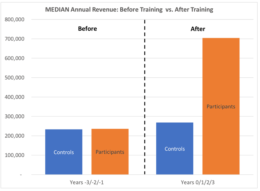
Figure 7 – Median Revenue: Contemporary Comparison
Retention Benefits? Participants remain with the firm at a higher rate
Not surprisingly, some attorneys disappear from our data after a certain year. We do not have information about why, but presumably, individuals leave the firm for retirement, another firm, another career, or another opportunity. Our analysis indicates that the participants were less likely to leave the firm relative to the set of control attorneys.
Figure 8 shows the percentage of Participant attorneys and Control attorneys in the Contemporary sample that remain visible in the data each year through 6 years after starting the program. Our data records go through 2017, so participants that began in later years will necessarily only be observed for a few years: e.g., the 2014 cohorts will only have three years of data post-program. For this figure, we focus only on the cohorts from 2007-2010, where participants have the opportunity to appear in the data for at least seven years after starting the program. The figure shows that all the participants remained in the data 6 years after the program began. By contrast, some control attorneys start disappearing from the data immediately, and by year 6, we have only 75% of the original matched controls.
One interpretation of this analysis is that participation in the program increases the likelihood that an attorney will stay with the firm.
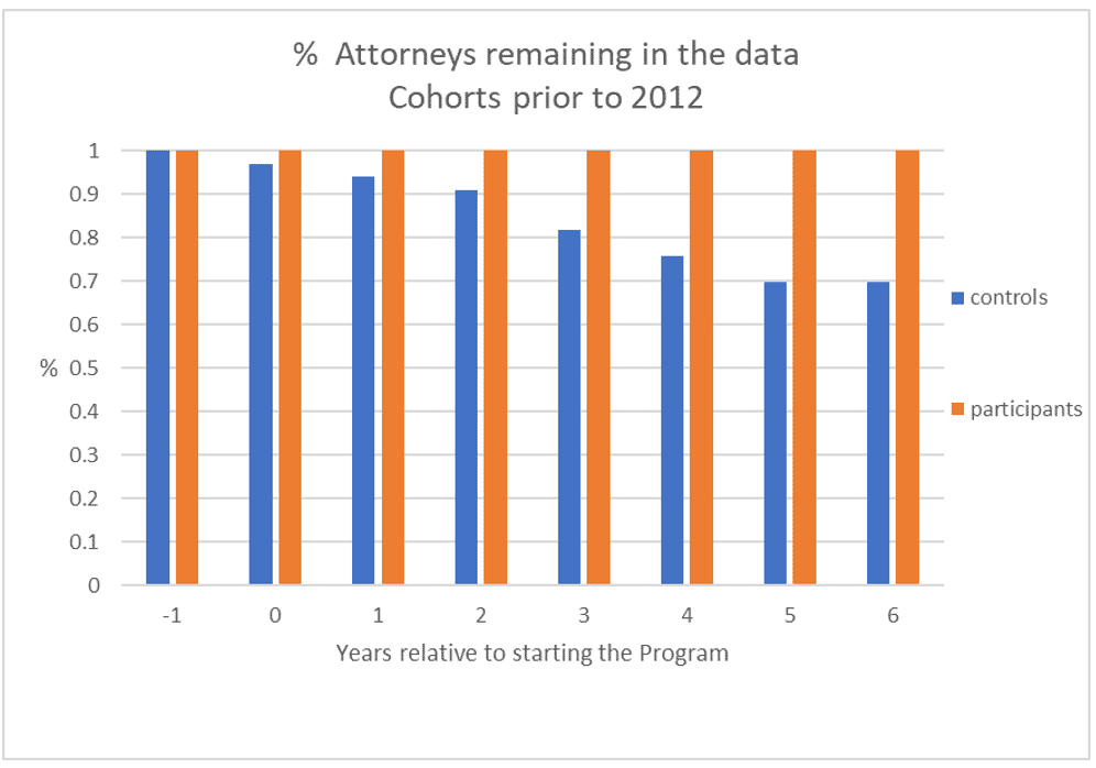
Figure 8 – Rate of Exit (Disappearance from data): Participants vs. Controls
After Three Years: Underperforming Control attorneys drop out
As noted earlier, we focused our analysis on the 3-year windows before and after the training program. This was to minimize the amount of attrition from our samples—i.e., the number of attorneys that disappeared from the data. As noted, these disappearances happen because we only had three years post-program for the last cohort in 2014 or because attorneys leave the firm.
Beyond the third post-program year, the average revenue of the contemporary controls begins catching up with the average revenue of the participants. This is not the case for the predecessor controls. For instance, in Figure 9, we show the estimated annual revenue impact of the program for the baseline -3 to +3 as well as for two longer time windows: +4 to +5. The estimated average annual revenue impact of the program declines noticeably for the Contemporaries comparison and a modest amount for the Predecessors comparison. (Note, though, that the estimated total impact of the program stays the same, even for the Contemporaries, as the lower annual average is offset by more years of higher revenue. For instance, for the Contemporary sample, the estimated annual impact times the number of years of impact is $971K for the -3-to-+3 window, but then $1.03M for the -3-to-+4 window and $991K for the -3-to-+5 window.)
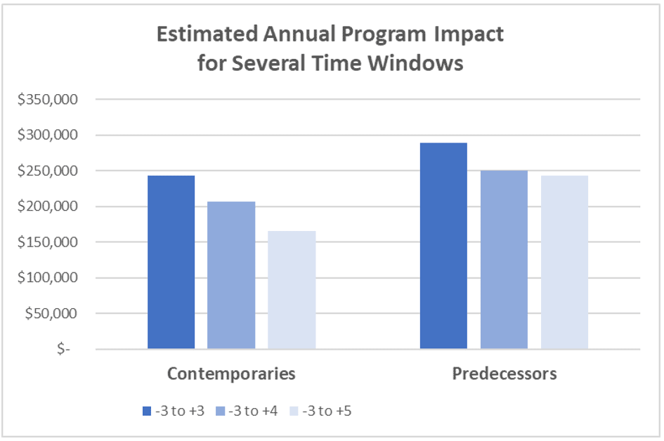
Figure 9 – Estimated Annual Impact for different lengths of time post-program
However, we noted earlier that the control attorneys drop out at a faster rate. It is important to point out that the contemporary control attorneys that drop out are low revenue producers, while those that remain are high revenue producers. For instance, in Figure 10, we show the average annual revenue of the contemporary controls that drop out during the 3-year “after” period vs. the average revenue of those that remain in the data for at least five years of the “after” period. The farther we look after the program start, the more than low-performing controls drop out, raising the control sample’s average revenue. So much of the “gain” by the control sample in later years comes from observing ever fewer, more successful attorneys. The comparison to the original set of participants becomes less-and-less apples to apples.
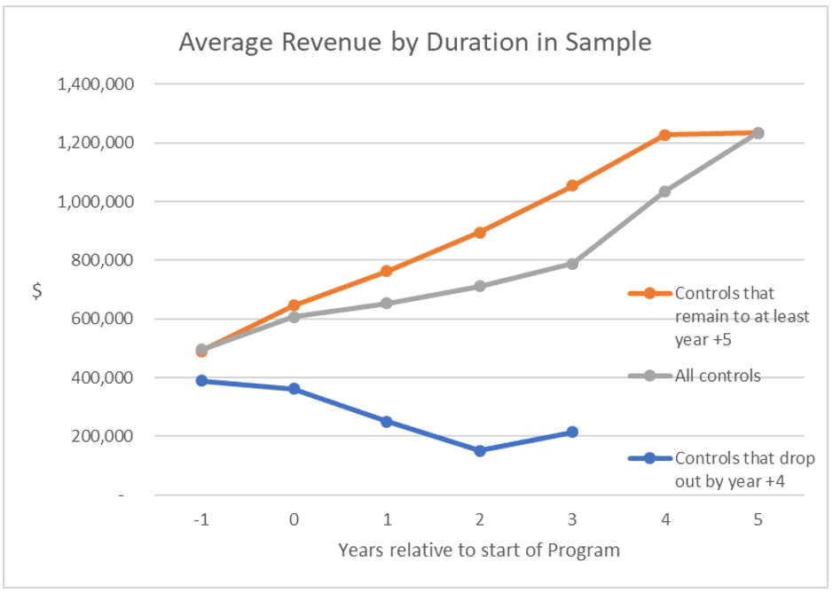
Figure 10 – Contemporary Controls that drop out of data are low performing
Summary of Program Impact Analysis:
To assess the effect of the BD program on participants’ business development success, we compared participants’ increase in revenue credits from the three years before to the three years after the program against the increase over the same period for two samples of non-participants: “contemporaries” who were similar to the participants in the year before starting the program; and “predecessors” who had the same characteristics as the participants in the 2002-2005 timeframe, before the first launch of the BD program.
Statistical analyses yielded an estimated impact of $244K (in the case of the contemporaries’ sample) and $288K (in the case of the predecessor sample) per participant per year for four years (the year the training began plus the three years after that). These point estimates represent the most likely average impact. The variance around each estimate suggests a 95% probability that the “true” impact lies between $22K per year and $481K per year.
There is evidence that the benefits of the BD program are spread widely among the participants, rather than being driven only by a few high-performing outliers, as the median revenue of participants also increases substantially—in contrast to the median revenue of the controls increases only very slightly.
There is also evidence that the BD program participants are less likely than non-participants to leave the firm, as indicated by the fact that attorneys in the control sample disappear from the firm’s data at a higher rate. The non-participants that drop out of the data also show lower average revenue levels (i.e., their average revenue declines in the “after” period). This means that the average revenue of the control sample increases more rapidly over time, as the sample consists of fewer but higher-performing attorneys. This partly accounts for the fact that the estimated advantage for participants gets narrower when we look beyond three years post-program.
Using the more conservative estimate of $244K per year for four years, the total estimated impact per participant is $976K. In other words, each participant-generated, on average, $976K in additional revenue that the firm would not have received without the program.
This Report and the following Technical Appendix are for Internal Management Use Only, not for distribution.
Copyright © 2019 Cochran Client Development, Inc., all rights reserved
Technical Appendix
Our Team Experience:
Dr. Heidi K. Gardner and Dr. Andrew von Nordenflycht are uniquely equipped to conduct this research. They have been actively researching the nature and benefits of collaboration in professional service firms for over a decade. Dr. Gardner has published the leading book on the subject (Smart Collaboration). They have worked with the internal records of several large law firms to address just these questions about collaboration: documenting the extent of collaboration and quantifying the client account benefits associated with it.
Heidi K. Gardner, Ph.D., is a Distinguished Fellow at Harvard Law School’s Center on the Legal Profession and author of the recently released book Smart Collaboration: How Professionals and Their Firms Succeed by Breaking Down Silos (Harvard Business Press). Dr. Gardner also serves as a Harvard Lecturer on Law and Faculty Chair of the school’s Accelerated Leadership Program. Previously she was a professor at Harvard Business School. Dr. Gardner has authored or co-authored more than fifty book chapters, case studies, and articles in scholarly and practitioner journals, including several in Harvard Business Review. Her first book, Leadership for Lawyers: Essential Strategies for Law Firm Success, was published in 2015.
Professor Gardner has lived and worked on four continents as a Fulbright Fellow and for McKinsey & Co. and Procter & Gamble. She earned her Master’s degree from the London School of Economics and her Ph.D. from London Business School. She was recently named by Thinkers 50 as a Next-Generation Business Guru.
Andrew von Nordenflycht, Ph.D., is an Associate Professor of Strategy at the Beedie School of Business at Simon Fraser University in Vancouver and an International Research Fellow with the Professional Service Firms Hub at Oxford’s Said Business School. He teaches MBA and Executive MBA courses in Strategy and Organizational Analysis. He publishes research on the challenges of governing and managing human capital-intensive firms, especially professional services. He works with executives and management teams to facilitate strategic analysis and strategic planning.
He received a BA from Stanford University (with distinction, Phi Beta Kappa) and a Ph.D. from the MIT Sloan School of Management. Before his academic career, he worked as a management consultant for The Monitor Group in Los Angeles and Boston.
Business Development Performance Measure: Revenue Credits
The Firm’s compensation system recognizes six types of revenue credit: client origination, client retention; client lead; matter origination; matter lead; and matter supervision. Each dollar of revenue the firm brings in gets counted six times in the compensation system for each type of credit. Each dollar of credit in each type can also be divided among multiple attorneys; e.g., $1 of client origination credit can be attributed 40% to one attorney and 60% to another.
To calculate each attorney’s annual revenue credit, we first added up the dollars of revenue credited to that attorney for each type across all matters. Then we combined the dollars across the six credit types using three different weightings.
The basic measure weighted each credit type equally, so the dollar value of each credit type was multiplied by (1/6), and those sums were added across credit types. (In effect, this was the same as adding up the total of each type and dividing by six.)
We also used two additional weightings. For “weighted revenue,” using the relative values of credits in the compensation system, where some credit types are more valuable than others (e.g., client lead was weighted 21.8%, while matter supervision was only 7.3%). For “origination revenue,” we only considered client origination and matter origination credits and weighted each at 50%. Figure 11 shows the three weightings.
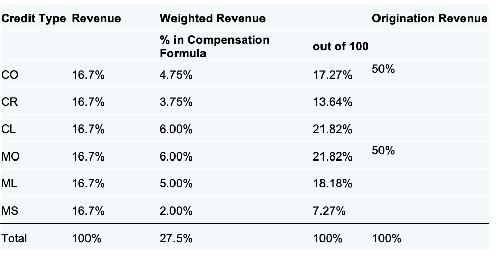
Figure 11 – Revenue Credit Weightings
The results were qualitatively similar across the three measures, so the report focuses on the primary, equally-weighted measure of revenue credit. Additionally, we use the term “revenue” instead of revenue credits throughout the report for brevity.
Regression Models
For the Contemporaries comparison, our regression model includes the following variables for each attorney in the sample:
Dependent variable: revenue. This is the annual revenue credits for a given attorney in a given year.
Independent variable: “participant X post-program” (the interaction of participant and post-program – see the list of Control variables below). This is a variable equal to 1 for observations of participants in the years after the program begins and 0 for all other observations. (In other words, it is equal to 0 for all observations of the non-participants and observations of the participants in the years before they began the program.).
Control variables:
- participant: This indicates whether the attorney was a participant or non-participant.
- post-program: This indicates whether the observation occurs in a year after the program began. For non-participants, this is determined by the program-start year for the participant to which they are matched.
- female: Set to 1 if the attorney is female, 0 if male.
- 15 office indicator variables: – for a given office, the indicator variable is set to 1 if the attorney was in that office, 0 otherwise.
For the Predecessors comparison, the regression model includes all the variables noted above and adds control variables for the calendar year. Specifically, it adds 16 indicator variables, one for each year from 2002-2017.
The regressions use ordinary least squares models. But non-participant observations are inversely weighted by their frequency with respect to the matched participant. In other words, where there is only one non-participant matched to a given participant, the non-participant is weighted as 1. But where three non-participants are matched to a given participant, the non-participants are weighted at 1/3.
Figure 12 shows the coefficient estimates and estimated probability that the actual coefficient is equal to zero.
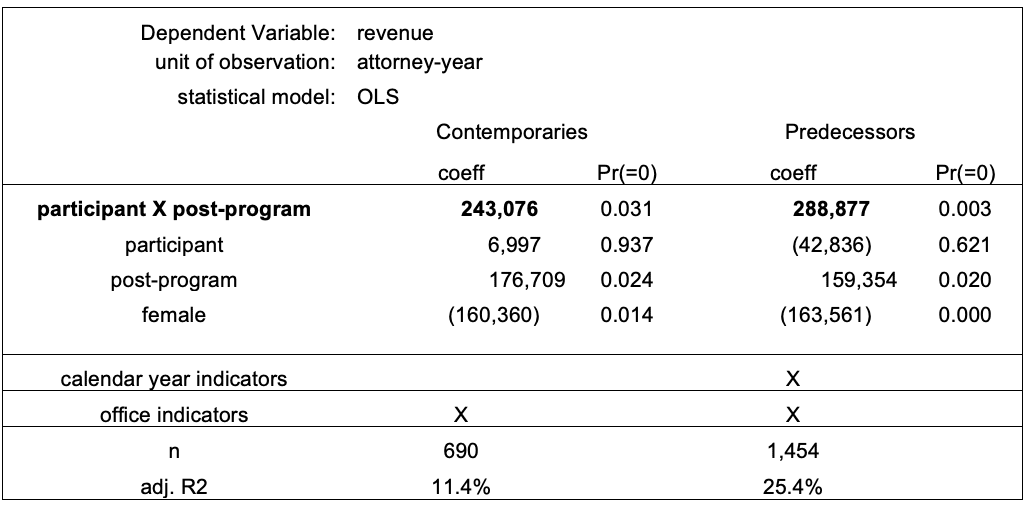
Figure 12 – Output from Statistical Models. (Note: Figures to right of coefficients are the probability that coefficient is equal to zero)
![]()
![]()
Austin | Boston | Chicago | London | Minneapolis | Seattle | Washington D.C.
© 2021-2026 – Cochran Client Development
